Tutorials
In this tutorial, we will go through different features of AMICAL. You can find a detailed description of the principal functions and associated parameters in their docstrings (easily accessible with good editors, e.g.: vscode).
- Step 1: clean and select data
- Step 2: extract observables
- Step 3: calibrate V2 & CP
- Step 4: analyse with CANDID and Pymask
In the following, we'll assume you imported the library as:
import amical
Step 1: clean and select data
The major part of data coming from general pipelines (applying dark, flat, distorsion, etc.) are not enought compliant with the Fourier extracting method developed within AMICAL.
The first step of running AMICAL consists in cleaning the data in different ways:
- Remove residual sky background (
sky=True,r1,dr) - Crop and center the image (
isz,f_kernel=3), - Apply windowing (
apod,window), - Apply bad pixels correction (
bad_map=None,add_bad=[],remove_bad=False).
We use a 2d gaussian interpolation to replace the bad pixels (same as
here). The keyword argument bad_map is
a 2D array (same shape as the data) filled with 0 and 1 where 1 stands for a bad
pixel (hot, cosmic, etc.). Instrument pipelines generally come with bad pixels
map generator, but you can add an unlimited number of bad pixels as the input
list add_bad (e.g.: [[24, 08], [31, 41]])).
nrm_file = "my_nrm_data.fits"

clean_param = {
    "isz": 69,  # final cropped image size [pix]
    "r1": 31,  # Inner radius to compute sky [pix]
    "dr": 2,  # Outer radius (r2 = r1 + dr)
    "apod": True,  # If True, apply windowing
    "window": 32,  # FWHM of the super-gaussian (for windowing)
}

# Firsly, check if the input parameters are valid
amical.show_clean_params(nrm_file, **clean_param)
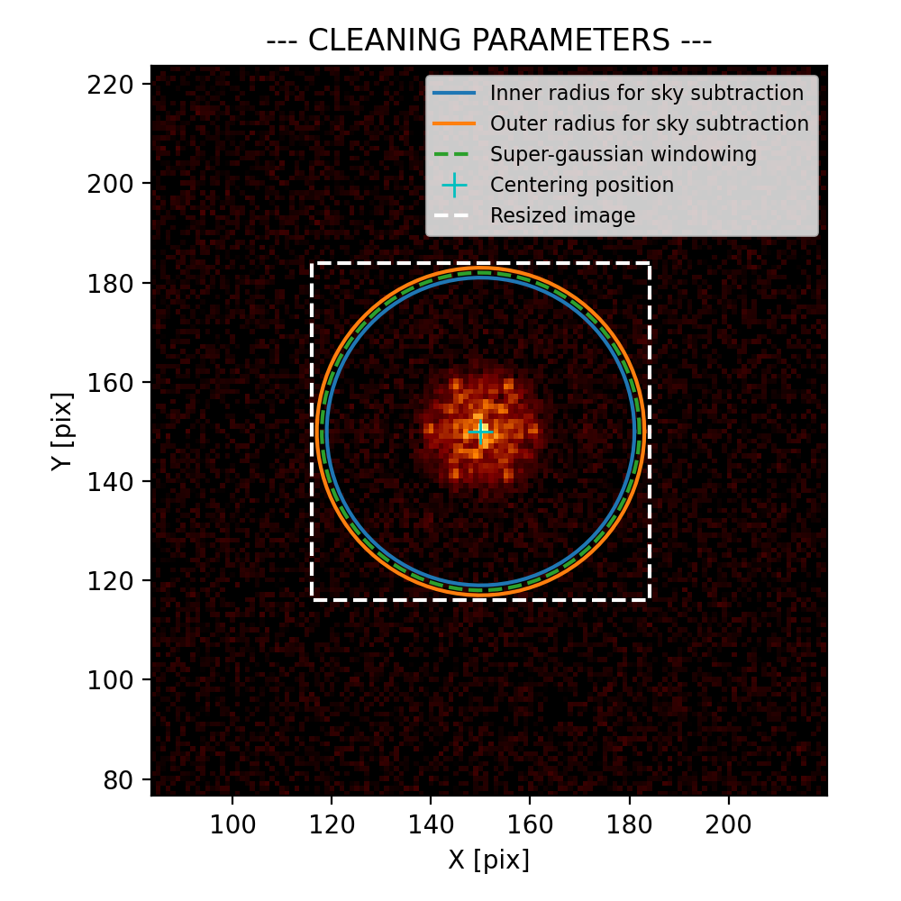
FIG. 1 - Example of appropriate set of parameters to clean NIRISS data.
If the cleaning parameters seem well located (cyan cross on the centre, sky radius outside the fringes pattern, etc.), we can apply the cleaning step to the data.
cube_cleaned = amical.select_clean_data(
    nrm_file, **clean_param, clip=True, clip_fact=0.5
)
During the cleaning step, you can decide to apply a lucky imaging selection
(clip=True) to accumulate only the best frames in the cube (based on the
integrated fluxes compared to the median: threshold = median(fluxes) -
clip_fact * std(fluxes)).
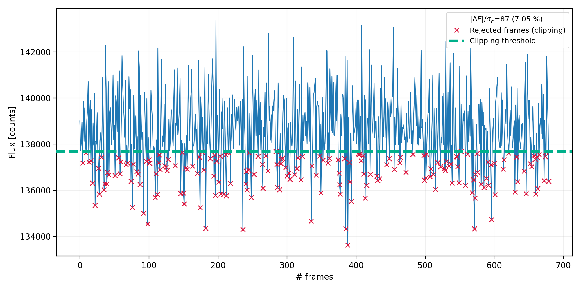
FIG. 2 - Example of integrated flux measurement along the cube (# frames). The rejected frames are labelled by the red cross. The threshold is represented with the green dashed line.
Step 2: extract observables
The second step is the core of AMICAL: we use the Fourier sampling approach to extract the interferometric observables (visibilities and closure phases).
The whole challenge when playing with the NRM data is to find the correct
position of each baseline in the Fourier transform. To do so, we implemented 4
different sampling methods (peakmethod = ('unique', 'square', 'gauss', 'fft'))
to exploit information spread beyond just the u, v positions (see
our SPIE 2020 reference
paper for more
details).
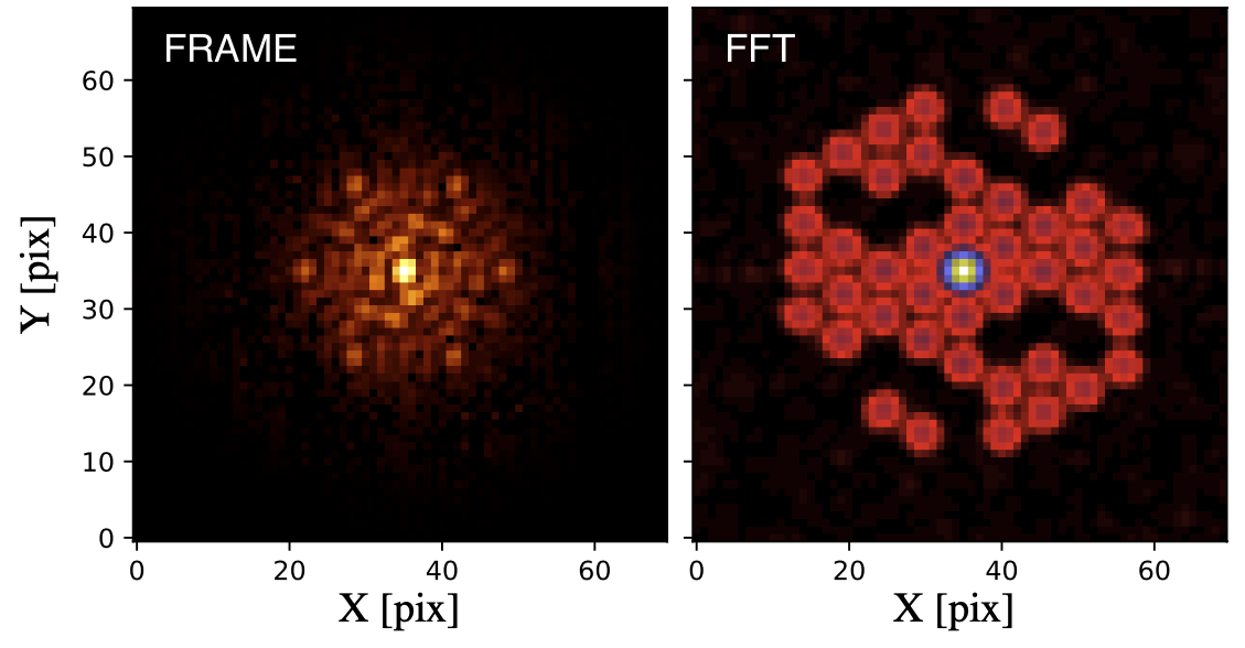
FIG. 3* - Example of NIRISS data. Left: Image plane representing the fringe pattern. Right:* Fourier transform (Fourier plane).

FIG. 4 - Zoom on one Fourier peak (called splodge) showing the different sampling methods.
Based on NIRISS and SPHERE dataset analysis, we recommend using the 'fft'
method (but feel free to test the other methods for your specific case!). The
expected baseline locations on the detector are computed using the mask
coordinates, the wavelength and the pixel size. In some cases, the mask is not
perfectly aligned with the detector and so requires to be rotated
(theta_detector = 0) or centrally scaled (scaling_uv = 1).
With AMICAL, the mask coordinates, the wavelengths, the pixel size and the
target name are normally read from the fits file header.
In case where headers are not compliant, you will need to provide the following keyword arguments: filtname, instrum and targetname.
params_ami = {
    "peakmethod": "fft",
    "maskname": "g7",  # 7 holes mask of NIRISS
}

bs = amical.extract_bs(cube_cleaned, file_t, **params_ami)
Note: Other parameters in
amical.extract_bs()are rarely modified but you can check the docstrings for details (bispect.py).
The object bs stores the raw observables (bs.vis2, bs.e_vis2, bs.cp,
bs.e_cp), the u-v coordinates and wavelength (bs.u, bs.v, bs.wl), the
baseline lengths (bs.bl, bs.bl_cp), information relative to the used mask
(bs.mask), the computed matrices and statistic (bs.matrix) and the important
information (bs.infos). The mask, infos and matrix attributes also hold various data.
print(bs.keys(), bs.mask.keys())
Step 3: calibrate V2 & CP
Closure phases and square visibilities suffer from systematic terms, caused by the wavefront fluctuations (temporal, polychromatic sources, non-zero size mask, etc.). To calibrate aperture masking data, these quantities are measured on one or several identified unresolved (or known size) calibration stars. In practice, we subtract the calibrator signal from the raw closure phases and normalize the target visibilities by the calibrator’s visibilities.
# bs_t and bs_c are the results from amical.extract_bs() on the target and
# calibrator respectively.
cal = amical.calibrate(bs_t, bs_c)
If several calibrators are available, the calibration factors are computed using
a weighted average to account for variations between sources. In this case,
bs_c will be a list of results from amical.extract_bs(). The extra errors
induced are then quadratically added to the calibrated uncertainties.
During the calibration procedure, a second data selection can be performed to
reject bad calibrator-source pairs using a sigma-clipping approach (clip=True,
using a threshold value in sigma sig_thres=2).
```python } cal = amical.calibrate(bs_t, [bs_c1, bs_c2, bs_c3], clip=True, sig_thres=2)
> Note: For ground based facilities, two additional corrections can be applied
> on V2 to deal with potential piston between holes (`apply_phscorr=True`) or
> seeing/wind shacking variations (`apply_atmcorr=True`). This functionnality
> was only tested on old dataset from the previous IDL pipeline, and so needs to
> be cautiously used (seem to not working on SPHERE data).

> Note: You can decide to normalize the CP uncertaintities by sqrt(n_holes/3)
> take into account the dependant vs. independant closure phases
> (`normalize_err_indep=True`).

Once again, `cal` is an object containing the calibrated observables
(`cal.vis2`, `cal.e_vis2`, etc.), u-v coordinates (`cal.u`, `cal.v`, `cal.u1`,
`cal.v2`, etc.), wavelength (`cal.wl`) and the output objects from step 2
(`cal.raw_t`, `cal.raw_c`).

You can now visualize the calibrated observables with `amical.show()` and save
them as the standard oifits file with amical.save().

```python
amical.show(cal, cmax=1, vmin=0.97, vmax=1.01)
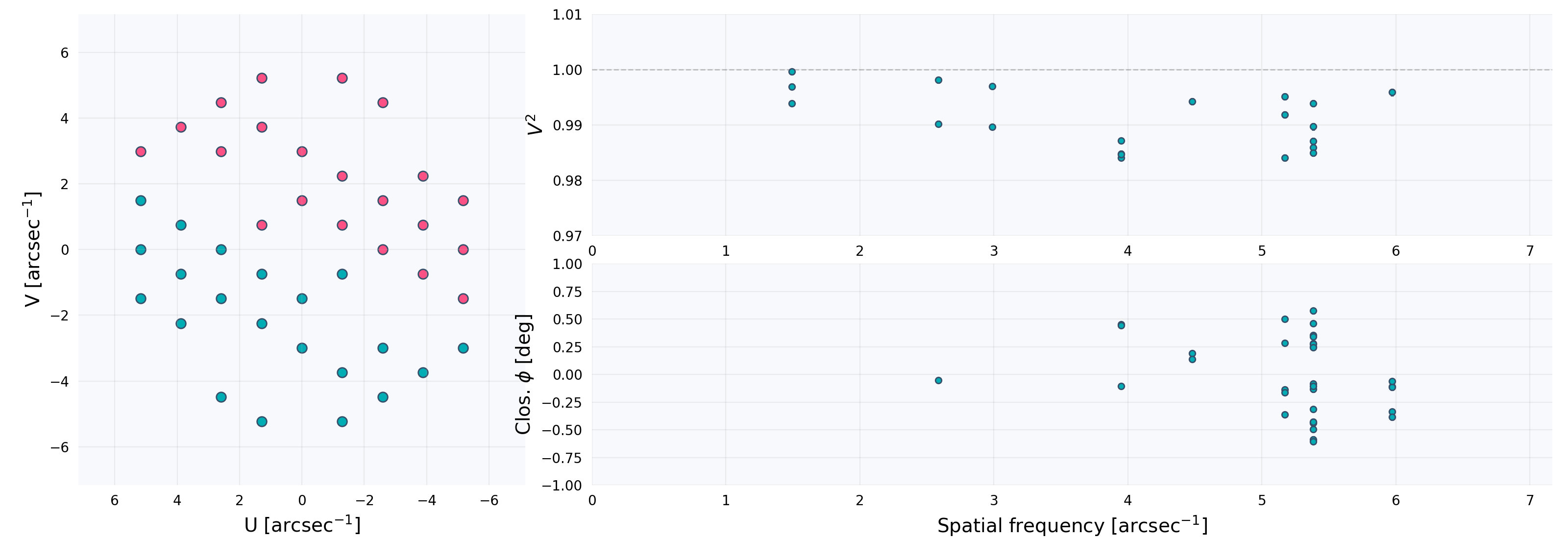
***FIG. 5** - Example of calibrated observables obtained with NIRISS. **Left:** u-v plan, **Top-right:** squared visibilities, **Lower-right:** Closure phases.* By default, we assume that the u-v plan is oriented on the detector (north-up, east-left) with `pa=0` in degrees. The true position angle is normally computed during the step 2 (not yet available for all instruments) and so need to be given as input with `pa=bs.infos.pa`. Few other parameters are available to set the axe limites (`vmax`, `vmin`, `cmax`), set units (`unit`, `unit_cp`), log scale (`setlog`), flags (`true_flag_v2`, `true_flag_cp`), etc.
oifits_file = "my_oifits_results.oifits"

amical.save(cal, oifits_file, pa=bs_t.infos.pa)
inputdata = "Saveoifits/my_oifits_results.oifits"

param_candid = {
    "rmin": 20,  # inner radius of the grid
    "rmax": 250,  # outer radius of the grid
    "step": 50,  # grid sampling
    "ncore": 12,  # core for multiprocessing
}

fit1 = amical.candid_grid(inputdata, **param_candid, diam=0, doNotFit=["diam*"])
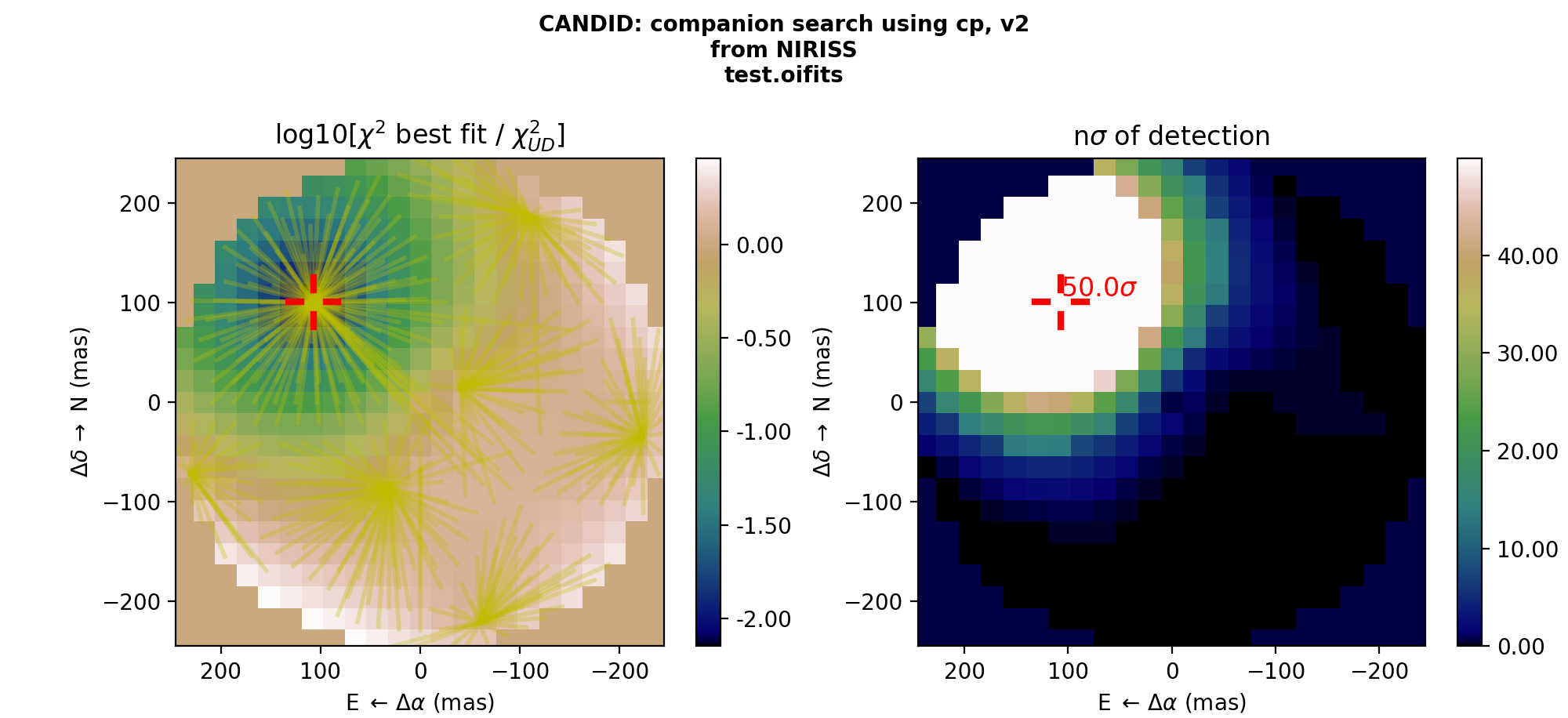
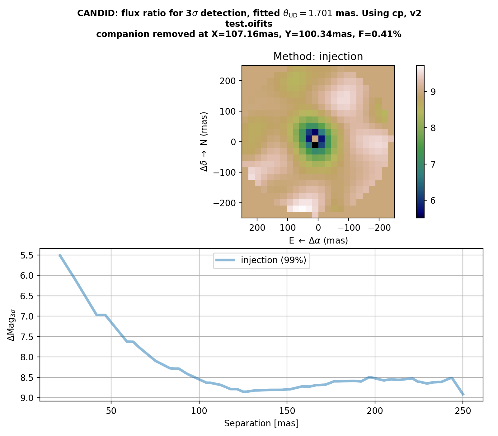
cr_candid = amical.candid_cr_limit(inputdata, **param_candid, fitComp=fit1["comp"])
